

[Hybrid Navigation System: Part 3 Hardware & Modeling] A Deep Dive into Industrial High-Performance INS & Making GPS Jamming Simulator
Hello! To all the university students and researchers pushing the boundaries of autonomous flight and unmanned navigation technologies—welcome back to QUAD Drone Lab.
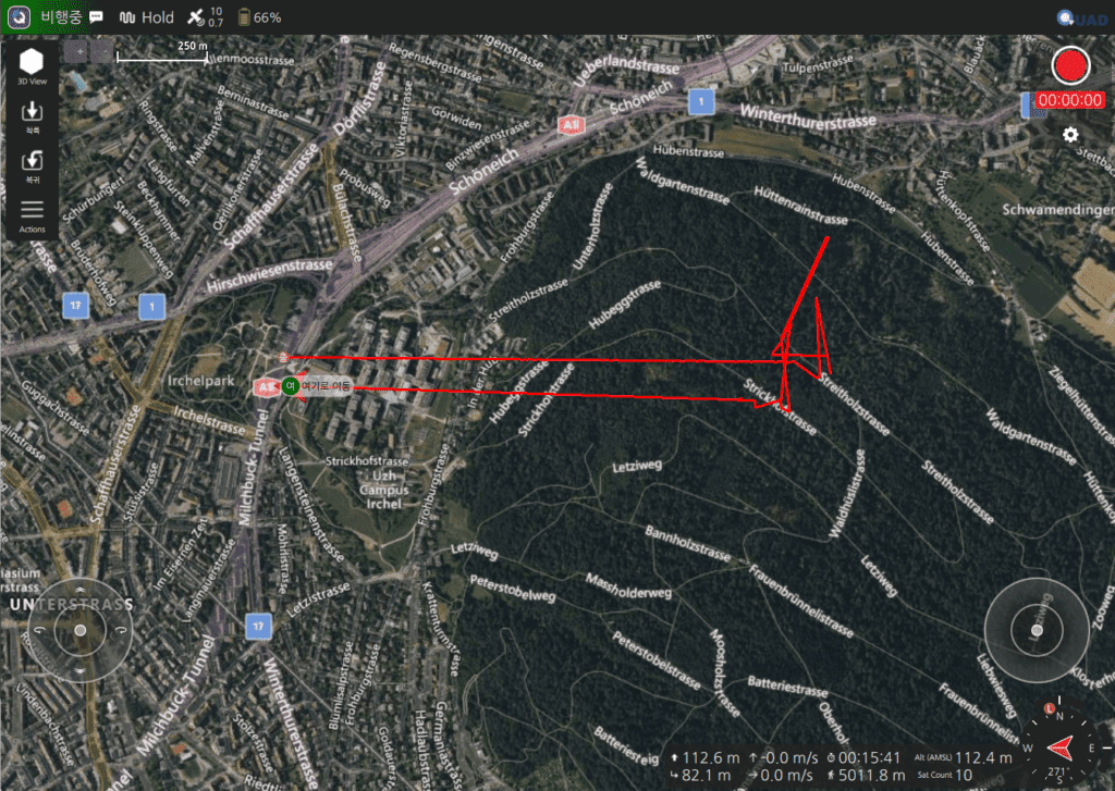
In our previous post, <Part 2>, we explored the state estimation principles of the PX4 EKF2 (the brain of our drone) and set up a safe Gazebo SITL simulator environment for testing. How did it feel flying the drone in the virtual world? When the GPS was on, it probably flew along its trajectory as smoothly as if it were on invisible rails.
However, what happens if you forcefully turn off the GPS in the simulator to mimic a GNSS-Denied environment? The drone immediately loses its sense of absolute position and slowly—or sometimes rapidly—begins to drift off course. This is the notorious ‘Drift’ phenomenon.
In this <Part 3> of our series, we will mathematically analyze the inherent limitations of standard low-cost sensors and why they fail at long-range ‘Dead Reckoning’. To overcome these limits, we will dive deep into the hardware technologies—specifically MEMS vs. FOG—of high-performance Industrial INS (Inertial Navigation Systems) used in real-world defense and aerospace. Finally, we will use Python to directly simulate the error drift based on different sensor grades.
Let’s get started!
1. The Greatest Enemy of Dead Reckoning: Double Integration and the Snowball Effect
When GPS is jammed or denied, a drone must rely entirely on its internal IMU (Inertial Measurement Unit). An IMU essentially consists of ‘gyroscopes’ that measure the rate of rotation and ‘accelerometers’ that measure linear acceleration.
The principle of calculating your position via dead reckoning is conceptually simple:
- Integrate the acceleration (a) measured by the accelerometer once to find the velocity (v). (v=∫adt)
- Integrate that velocity once more to find the position (p). (p=∫vdt)
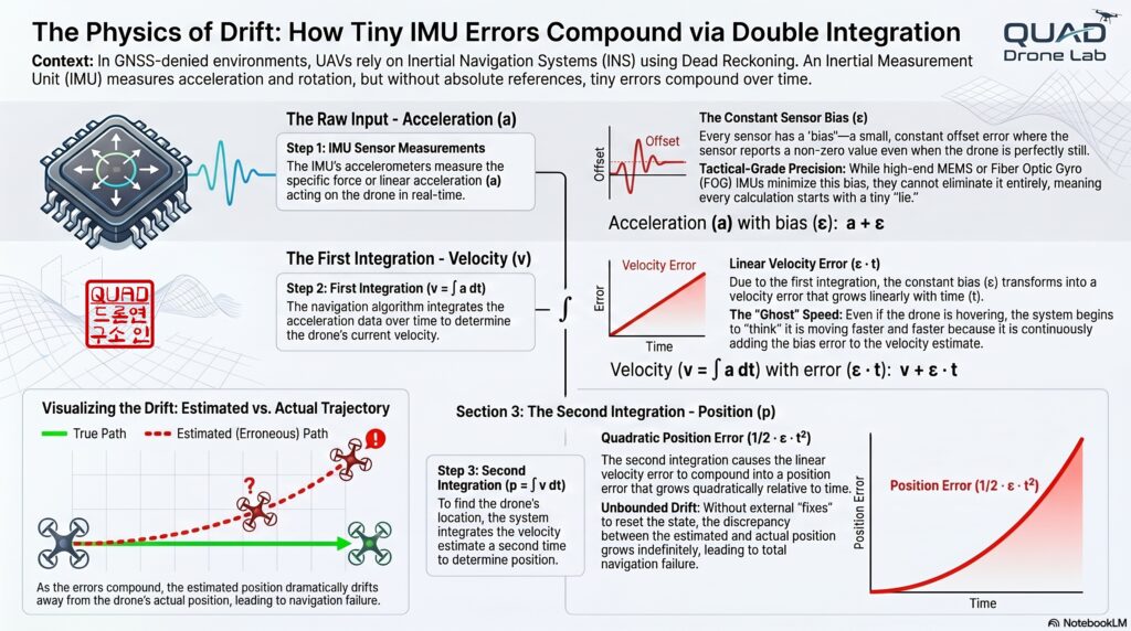
The fatal flaw is that real-world sensor data always contains ‘Noise’ and ‘Bias’ (a constant offset from zero). Imagine there is a tiny, constant bias error ϵ mixed into your acceleration data.
- Velocity Error: ∫ϵdt=ϵt (grows proportionally with time)
- Position Error: ∫ϵtdt=21ϵt2 (grows exponentially with the square of time)
Furthermore, if the gyroscope has a slight angular error, the drone will miscalculate its tilt. This causes the massive force of Earth’s gravity to be incorrectly projected as horizontal acceleration. Because of this, the position error will actually explode proportionally to the cube of time (t3)! This is why a $1 smartphone IMU will drift tens or hundreds of meters within just 60 seconds of losing GPS.
2. Deep Dive into Hardware: MEMS vs. FOG Technology
For a kamikaze UAV to fly hundreds of kilometers and strike a target without GPS, we need a high-performance Inertial Navigation System (INS) that can drastically slow down this error accumulation. Industrial and tactical INS sensors are primarily divided into two technologies: FOG and MEMS.
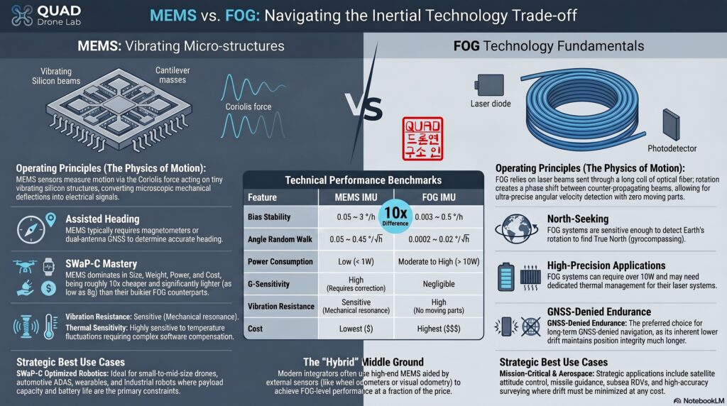
📍 FOG (Fiber Optic Gyroscope)
- Principle: FOGs use the ‘Sagnac Effect’. They send beams of light in opposite directions through a coiled optical fiber; when the sensor rotates, the light traveling against the rotation takes a slightly different amount of time to exit the coil compared to the light traveling with it.
- Features: Because they have no moving parts or mechanical friction, they are highly resistant to vibration and offer ultra-precision. They are typically used in submarines, large aircraft, and long-range cruise missiles.
- Drawbacks: To achieve high precision, you need a long coil of fiber, making these sensors large, heavy (often several kilograms), and very expensive (tens of thousands of dollars). From a SWaP-C (Size, Weight, Power, and Cost) perspective, they are usually too bulky for small kamikaze drones. (Note: This specific SWaP-C analysis is based on general aerospace engineering principles outside the provided text).
📍 MEMS (Micro-Electro-Mechanical Systems)
- Principle: MEMS technology uses microscopic silicon structures. When the system rotates, a vibrating proof mass experiences a Coriolis force. This force induces a secondary vibration whose amplitude is directly proportional to the angular velocity, which is measured as a change in capacitance by specialized readout circuits.
- Features: They are ultra-compact, extremely lightweight (tens of grams), low-power, and affordable due to mass production.
- Drawbacks & Evolution: Historically, MEMS sensors were noisy and relegated to consumer electronics. However, rapid advancements in microelectronics and calibration algorithms have revolutionized them. Today, ‘Tactical Grade’ MEMS INS exist that rival the performance of older FOG systems.
💡 Sensor Selection Guide for Kamikaze Drones
Unlike returning aircraft, kamikaze or small reconnaissance drones need sensors that balance high performance with strict SWaP-C constraints. Therefore, High-End Tactical MEMS INS are the optimal choice. Market-leading products include the SBG Systems Ekinox Micro (which combines tactical MEMS with quad-constellation GNSS in a rugged, miniature form), the MicroStrain 3DM-GQ7 (a tactical-grade INS with RTK), and the Honeywell HG4930 MEMS IMU. These sensors, weighing well under 100g, feature embedded Extended Kalman Filters (EKF) that suppress drift to just a few meters even during extended GNSS outages.
3. [Hands-on] Python Simulation of Position Drift by INS Grade
Seeing is believing. Let’s write a Python simulation to visually compare how the position error diverges during dead reckoning based on the grade of the sensor.
We will build a 1D double-integration model using two critical specs found on sensor datasheets: Bias Instability and Velocity Random Walk (White Noise).
[Requirements] A Python environment with numpy and matplotlib installed.
import numpy as np
import matplotlib.pyplot as plt

def simulate_ins_1d(duration_sec, dt, accel_bias_mg, velocity_random_walk):
    """
    Simulates dead reckoning position error based on sensor noise in a 1D flight.
    :param duration_sec: Total flight time without GPS (seconds)
    :param dt: Sampling time (seconds)
    :param accel_bias_mg: Accelerometer bias (mg, 1mg = 0.001g)
    :param velocity_random_walk: Velocity Random Walk noise (m/s/sqrt(hr))
    """
    g = 9.80665  # Gravity (m/s^2)
    n_steps = int(duration_sec / dt)
    time = np.linspace(0, duration_sec, n_steps)

    # 1. Assume the drone is flying straight at a constant speed (True Acceleration = 0)
    true_accel = np.zeros(n_steps)

    # 2. Convert sensor specs to standard SI units
    bias_m_s2 = (accel_bias_mg / 1000.0) * g
    # Convert VRW to discrete time standard deviation: (m/s/sqrt(hr)) -> (m/s^2)
    noise_std_dev = (velocity_random_walk / 60.0) * (1 / np.sqrt(dt))

    # 3. Generate Accelerometer Measurements (True + Bias + White Noise)
    noise = np.random.normal(0, noise_std_dev, n_steps)
    measured_accel = true_accel + bias_m_s2 + noise

    # 4. Dead Reckoning (Double Integration: Accel -> Vel -> Pos)
    estimated_vel = np.zeros(n_steps)
    estimated_pos = np.zeros(n_steps)

    for i in range(1, n_steps):
        estimated_vel[i] = estimated_vel[i-1] + measured_accel[i] * dt
        estimated_pos[i] = estimated_pos[i-1] + estimated_vel[i] * dt

    return time, estimated_pos

# --- Simulation Parameters ---
duration = 600  # Assume GPS is jammed for 10 minutes (600 seconds)
dt = 0.01       # 100Hz sampling rate

# 1. Low-cost Consumer IMU (Smartphone / Toy Drone grade)
# Accel Bias: ~2mg, VRW: 0.1 m/s/sqrt(hr)
time, pos_consumer = simulate_ins_1d(duration, dt, accel_bias_mg=2.0, velocity_random_walk=0.1)

# 2. Tactical Grade MEMS INS (Ideal for Kamikaze Drones)
# Accel Bias: ~0.05mg, VRW: 0.02 m/s/sqrt(hr)
time, pos_tactical = simulate_ins_1d(duration, dt, accel_bias_mg=0.05, velocity_random_walk=0.02)

# 3. Navigation Grade FOG (Cruise Missile grade)
# Accel Bias: ~0.005mg, VRW: 0.005 m/s/sqrt(hr)
time, pos_nav = simulate_ins_1d(duration, dt, accel_bias_mg=0.005, velocity_random_walk=0.005)

# --- Visualization ---
plt.figure(figsize=(10, 6))
plt.plot(time, pos_consumer, label="Low-cost Consumer IMU Error", color='red')
plt.plot(time, pos_tactical, label="Tactical MEMS INS Error", color='blue', linewidth=2)
plt.plot(time, pos_nav, label="Navigation Grade FOG Error", color='green', linewidth=2)

plt.title("Position Drift Over Time Without GPS (10 Minutes)")
plt.xlabel("Time (seconds)")
plt.ylabel("Position Error (meters)")
plt.legend()
plt.grid(True)
plt.show()
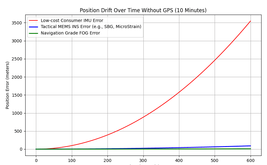
[Code Analysis & Results] When you run this code, the results are eye-opening. Even though the drone is mathematically flying at a constant speed, the double integration of tiny accelerometer errors causes the Consumer IMU (Red Line) to drift by hundreds or even thousands of meters in just 10 minutes, forming a massive quadratic curve.
In stark contrast, the Tactical MEMS INS (Blue Line)—the type of hardware we are adopting—exhibits a much gentler curve, successfully keeping the error down to just a few tens of meters over the same 10-minute window. The Navigation Grade FOG (Green Line) stays practically flat.
This simple experiment gives us a definitive answer to the question: “Why must we spend thousands of dollars on a tactical MEMS INS for long-range autonomous drones?”
4. Modeling Sensor Noise in the Gazebo SITL Environment
The mathematical model we just verified using Python can also be applied to the Gazebo SITL simulator we set up in Part 2. To make the virtual drone in the simulator exhibit the same error characteristics as a real-world industrial drone, we need to modify the settings of the imu_sensor plugin.
I have modified the following files to enable real-time control of GPS noise within the PX4 simulation. The primary goal was to add noise to the navsat sensor of the Gazebo model and implement dynamic parameters in the PX4 GPS simulation module.
Drone’s IMU(INS)
/home/quad/PX4-Autopilot/Tools/simulation/gz/models/x500_base/model.sdf
      <sensor name="imu_sensor" type="imu">
        <always_on>1</always_on>
        <update_rate>250</update_rate>
        <imu>
          <angular_velocity>
            <x>
              <noise type="gaussian">
                <mean>0</mean>
                <stddev>0.0000436</stddev> <!-- 자이로 ARW -->
                <dynamic_bias_stddev>0.00000727</dynamic_bias_stddev> <!-- 자이로 바이어스 불안정성 -->
                <dynamic_bias_correlation_time>400.0</dynamic_bias_correlation_time>
              </noise>
            </x>
            <y>
              <noise type="gaussian">
                <mean>0</mean>
                <stddev>0.0000436</stddev>
                <dynamic_bias_stddev>0.00000727</dynamic_bias_stddev>
                <dynamic_bias_correlation_time>400.0</dynamic_bias_correlation_time>
              </noise>
            </y>
            <z>
              <noise type="gaussian">
                <mean>0</mean>
                <stddev>0.0000436</stddev>
                <dynamic_bias_stddev>0.00000727</dynamic_bias_stddev>
                <dynamic_bias_correlation_time>400.0</dynamic_bias_correlation_time>
              </noise>
            </z>
          </angular_velocity>
          <linear_acceleration>
            <x>
              <noise type="gaussian">
                <mean>0</mean>
                <stddev>0.000196</stddev> <!-- 가속도계 VRW -->
                <dynamic_bias_stddev>0.000049</dynamic_bias_stddev> <!-- 가속도계 바이어스 불안정성 -->
                <dynamic_bias_correlation_time>400.0</dynamic_bias_correlation_time>
              </noise>
            </x>
            <y>
              <noise type="gaussian">
                <mean>0</mean>
                <stddev>0.000196</stddev>
                <dynamic_bias_stddev>0.000049</dynamic_bias_stddev>
                <dynamic_bias_correlation_time>400.0</dynamic_bias_correlation_time>
              </noise>
            </y>
            <z>
              <noise type="gaussian">
                <mean>0</mean>
                <stddev>0.000196</stddev>
                <dynamic_bias_stddev>0.000049</dynamic_bias_stddev>
                <dynamic_bias_correlation_time>400.0</dynamic_bias_correlation_time>
              </noise>
            </z>
          </linear_acceleration>
        </imu>
</sensor>GPS Jamming
I have modified the following files to enable real-time control of GPS noise within the PX4 simulation. The primary objective was to inject noise into the navsat sensor of the Gazebo model and implement dynamic parameters into PX4’s GPS simulation module.
Target Files:
/src/modules/simulation/sensor_gps_sim/parameters.c/src/modules/simulation/sensor_gps_sim/SensorGpsSim.hpp/src/modules/simulation/sensor_gps_sim/SensorGpsSim.cpp
1. parameters.c
- Modification: Added new GPS noise parameters.
- Details:
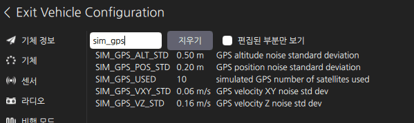
SIM_GPS_POS_STD: Horizontal position noise standard deviation (Default: 0.2m, Range: 0–100m)SIM_GPS_ALT_STD: Altitude noise standard deviation (Default: 0.5m, Range: 0–100m)SIM_GPS_VXY_STD: XY velocity noise standard deviation (Default: 0.06m/s, Range: 0–100m/s)SIM_GPS_VZ_STD: Z velocity noise standard deviation (Default: 0.158m/s, Range: 0–100m/s)
- Purpose: Parameterizing GPS noise so it can be adjusted in real-time via QGroundControl (QGC).
2. SensorGpsSim.hpp
- Modification: Added definitions for the new parameters.
- Details: Included the four parameters mentioned above within the
DEFINE_PARAMETERSmacro. - Purpose: Declaring parameters in the header file for module integration.
3. SensorGpsSim.cpp
- Modification: Updated GPS noise calculation to be parameter-based.
- Details:
- Latitude/Longitude noise: Utilized
_sim_gps_pos_std.get(). - Altitude noise: Utilized
_sim_gps_alt_std.get(). - Velocity noise: Utilized
_sim_gps_vxy_std.get()and_sim_gps_vz_std.get(). - Fixed type casting issues (resolved float to double conversion warnings).
- Latitude/Longitude noise: Utilized
- Purpose: Replaced hard-coded noise values with dynamic parameters to allow real-time tuning during flight simulation.
This creates a perfect testbed, allowing us to determine exactly when and where our visual Terrain Matching algorithm (Stage 2) needs to intervene to reset this accumulated drift.
With these modifications, we can now dynamically test GPS noise in real-time while the simulator is running.
Wrapping Up
In this <Part 3>, we unraveled the mathematical nightmare of dead reckoning (the snowball effect of double integration) and highlighted the absolute necessity of Industrial High-Performance INS (Tactical MEMS) hardware. Through our Python simulation, we visualized exactly how numbers on a datasheet translate into catastrophic or manageable flight trajectories.
However, even with an expensive tactical MEMS INS, flying hundreds of kilometers will eventually result in hundreds of meters of drift. Hardware alone is not a silver bullet.
Therefore, in our next post, <Part 4>, we will explore the practical software integration architecture. We will learn how to take the hyper-precise Odometry data output by these external high-performance INS modules and inject it directly into the PX4 flight control loop using the ROS 2 Communication Bridge.
Get ready to connect the brain and the sensory organs of our kamikaze drone in the next installment!

Author: maponarooo, CEO of QUAD Drone Lab
Date: April 17, 2026
![[Series Announcement] ROS2 Mastery: A Comprehensive ROS2 Guide for Students and Researchers](https://quad-drone-lab.co.kr/wp-content/uploads/2026/03/image-11-768x429.png)
![[Hybrid Navigation System Series Part 1: Overview] Flying Hundreds of Kilometers Without GPS? Learning a Hybrid Navigation System from WWII Pilots](https://quad-drone-lab.co.kr/wp-content/uploads/2026/04/컴패니언-컴퓨터-기반의-AI-지형지물-보정-768x419.jpg)